New to paleoclimate, or to the climate of Alaska? Find some key concepts explained below!
Climate of South Alaska
South Alaska is an interesting and important place to study climate change. This is in part due to its location in the sub-arctic latitudes, which are being strongly impacted by current global warming relative to more temperate and tropical regions. The pronounced impact of modern warming has caused dramatic changes in the environment, such as rapidly melting glaciers, which are important to understand along with their climatological context. South Alaska is also strongly impacted by atmospheric and oceanic systems of the North Pacific Ocean. This is significant because these same systems also impact the climate all along the North Pacific eastern continental margin, from Alaska to southern California, but are most easily measured in south-central Alaska due to their particularly strong signals in that region.
The most important of these systems are:
1) The Aleutian Low atmospheric pressure cell
2) The Pacific Decadal Oscillation
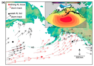
The Aleutian Low (AL) is a zone of low sea-level pressure that strengthens (lower pressure) each winter and weakens (higher pressure) in the summer. The center of the wintertime, strengthened low-pressure zone tends to be in the Gulf of Alaska. This means that moisture is drawn toward the Gulf of Alaska and south-central Alaska from the south, resulting in relatively stormy and wet conditions in the wintertime. In the summer, the low-pressure zone becomes less pronounced, and often splits into two nodes: one near the Aleutian Islands, and one near southwestern Yukon. Therefore, storms are more likely to travel over the Alaskan landmass before being arriving in south-central Alaska, and are generally less strong.
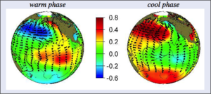
In addition to this seasonal change in the AL, the pressure zone also periodically strengthens and weakens over longer time scales; the AL could be relatively strong for a few decades, and then weaken for a few decades. In other words, the AL can shift multi-decadally. Therefore, there are multi-decadal periods that are relatively stormier than others in south-central Alaska. These longer-term shifts in the AL are thought to be impacted by the Pacific Decadal Oscillation (PDO), which is a pattern of sea-surface temperature changes that also occurs on a multi-decadal timescale. A warm phase of the PDO is characterized by warm sea surfaces in the eastern part of the North Pacific Ocean, while the cool phase is the opposite. These longer term changes in the AL and PDO impact the entire Pacific coast of North America to varying degrees, and are important to study, and these changes are most easily measurable in south-central Alaska due to their more pronounced impacts.
Lake sediment cores and paleoclimate
Paleoclimatology is the study of climate of the past, and paleoclimatologists often study changes in climate conditions over several thousands of years in the past. In this project, we focus primarily on “the Holocene,” or the current interglacial period which began ~12,000 years ago when ice sheets receded in the Northern Hemisphere following the last glacial period. It is important to study paleoclimatology for a variety of reasons, such as:
1) To better understand the natural variability of complex climate systems by studying their behavior over long time scales
2) To find previous periods of climate warming, or “climate analogs,” to help understand environmental responses we may experience under current global warming
3) To put modern global warming into a broader context; is our current predicament truly unusual?
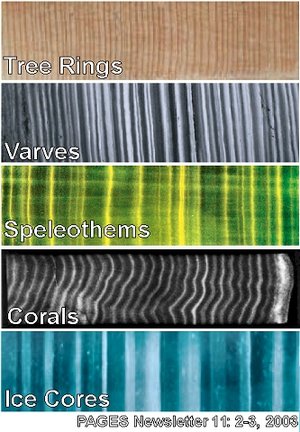
To answer questions like these, paleoclimatologists use a variety of natural climate archives, or places on earth that naturally record changes in climate conditions. One of the most common types of climate archives is tree rings: as trees grow, they create annual rings that can be measured and studied to reconstruct the climate conditions in which that tree grew over time. For example, thicker tree rings might be related to warm temperatures or increased precipitation, depending on the type of environment in which the tree grows. There are many other types of natural climate archives, including corals, stalagmites, ocean sediment cores, and lake sediment cores.
The “South Alaska Lakes” project utilizes lake sediment cores. As plant, animal, and mineral matter sinks to the bottom of a lake, these materials settle on the lake floor and accumulate vertically over time, bringing with them valuable information of climate conditions. By coring the lake sediments, which often extend several meters from the most recent (at the water) to the oldest materials (at the bedrock underlying the lake), we can collect a sequence of lake sediments that have been deposited over a long time—often thousands of years! Depending on the research question at hand, different aspects of the lake sediments can be studied, including: -fossil pollen, which can be identified and taxonomically classified, and used to reconstruct changes in vegetation -sediment grain sizes, which can be used to reconstruct flood frequency, glacial activity, and other depositional events -geochemical indicators, such as changes in stable isotopes of shells, organisms, or plant matter, which can be to reconstruct changes in precipitation patterns
Two types of lake sediment core analyses we use in this project are varve thickness and diatom oxygen isotopes, as explained below.
Varves
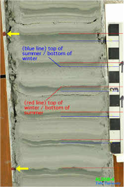
Varves are the lake sediment equivalent of tree rings; they are annually deposited layers that represent seasonal variations, with varying thicknesses depending on climate conditions. However, varves do not form in all lakes. Only lakes that are relatively deep, so that the lake floor remains undisturbed, are capable of forming varves. Varves are particularly common in glacial lakes, where the lake surface is frozen for a large portion of the year, and there is a distinctive pulse of glacial meltwater in the spring. Varves form from the contrast between this spring melt, which is lighter in color and comprised of silty material from fluvially transported sediments, and the frozen part of the year, which is darker in color and composed of settling organic matter in the still lake waters. Variations in the thickness of these varves can be related to climate conditions that drive larger glacial melt, such as temperature and precipitation. This type of study is currently in motion at Eklutna and Skilak Lakes.
Diatom oxygen isotopes
Every element on the periodic table has at least one isotope. You can think of isotopes as slightly different versions of the same chemical element, almost like sub-species within a species of animal or plant. You might recall that an atom contains protons (positive charge), electrons (negative charge), and neutrons (no charge). The only difference between, for example, one isotope of oxygen and other, is the number of neutrons. 16 O, 17 O, and 18 O, all have a different number of neutrons, as reflected by the different numbers. That means that there is an ever so slight difference in the mass of these various isotopes; 18 O is a bit heavier than 16 O, because of its extra neutrons.
Through advanced geochemical methods, it’s possible to measure changes in the relative abundance of 18 O to 16 O ( 17 O occurs in such low abundances that it’s very difficult to measure). Changes in this abundance are influenced by changes in climate conditions. For example, in lakes without major inflows and outflows (“closed” systems), the oxygen isotopes in the lake water are influenced heavily by evaporation. This is because 16 O evaporates more easily than 18 O. Therefore, in relatively dry periods when more evaporation occurs, lake water will be enriched in 18 O, because more 16 O will have evaporated from the lake surface.
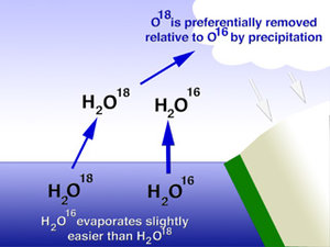
In “open” lakes, where water cycles through the lake relatively quickly due to larger inflows and outflows, lake water oxygen isotopes tend to reflect changes in precipitation isotopes. For example, when a storm travels from the Gulf of Alaska during a strong AL, it tends to contain relatively more 18 O compared to a storm that travels across the Alaskan interior during a weak AL. This is because 18 O tends to condense into precipitation more than 16 O; following this logic, the more precipitation that occurs (for instance, as a storm travels over Alaska), the less 18 O the remaining precipitation contains. Therefore, an “open” lake should contain relatively heavier (more 18 O) oxygen isotopes in a strong AL, and relatively lighter (more 16 O) during a weak AL. It is common to study oxygen isotope records in lake sediments using this logic, as we are doing in the “South Alaska Lakes” project.
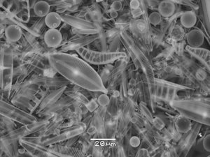
In this project, oxygen isotopes are being measured as they were recorded in diatoms. Diatoms are a large taxonomic group of freshwater algae comprised of biogenic silica (silica and oxygen). Therefore, we are purifying diatom skeletons (or frustules) in lake sediments in order to analyze the oxygen isotopes in both “closed” and “open” lakes to study both changes in evaporation and in AL behavior over time.